Supply Shock, predicting price by quantifying intent to buy and sell
Introduction
In any market, price is driven by demand and supply. This is a fundamental.
The most obvious way of seeing this is in the bid and asks between buyers and sellers. A more nuanced way would be to wave a magic wand and gauge the intent of investors before the bids and offers are even placed. In this view of demand and supply, an investor who has no intention to sell is on the demand side while an investor who is willing to sell is on the supply side.
This turns out to be a very simple equation to quantify which I've called "Supply Shock".
Supply Shock = unavailable supply / available supply
This is because the available and unavailable supply carry intent.
Quantifying Supply Shock
The Supply Shock equation can have multiple quantitative interpretations, each being a different take in estimating coins that are unavailable and available respectively.
Here are some examples:
- Exchange Supply Shock: Coin supply not available in self-custody storage vs coin supply available on exchanges
- Liquid Supply Shock: Coins held by investors with a history of accumulating vs coins held by speculative investors with a history of buying and selling
- Long Term Holder Supply Shock: Coins that have not moved in a long time and therefore considered unavailable vs coins that have been recently moved and therefore considered more available.
This is not an exhaustive list, but it will give you an idea of different ways to quantify this family of metrics.
Modelling Supply Shock
The version of Supply Shock I like the most is Liquid Supply Shock as it captures investor intent very well.
Glassnode’s Liquid Supply metric forensically clusters wallet addresses into distinct investors and then classifies their coins as illiquid, liquid or highly liquid based on the historic behaviour of the investor.
Using this data we can run the Supply Shock ratio as:
Liquid Supply Shock = Illiquid Coins / (Liquid + Highly Liquid Coins)
The chart below is the result.
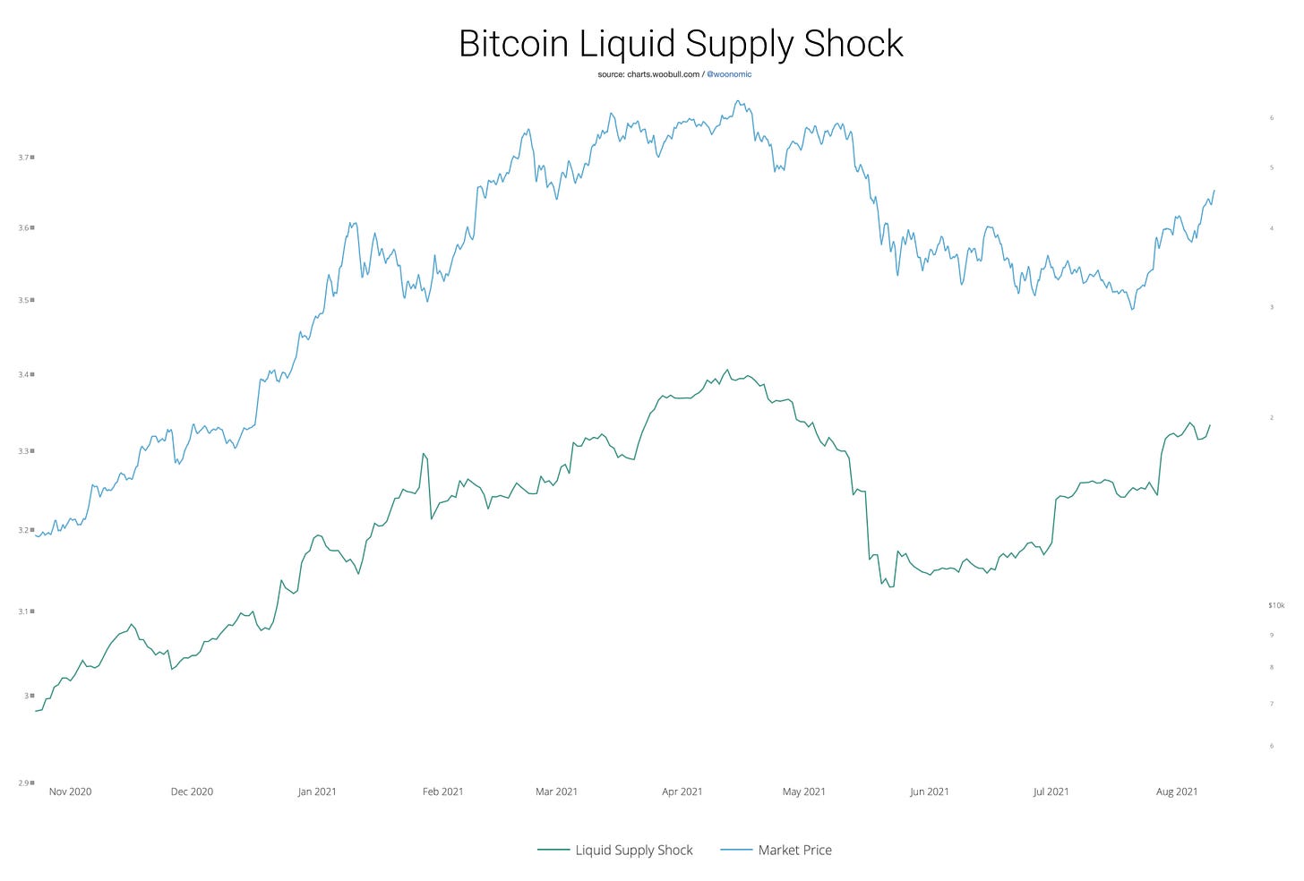
At first glance you can see the Supply Shock model tracks price quite closely. A closer look shows Supply Shock LEADS price.
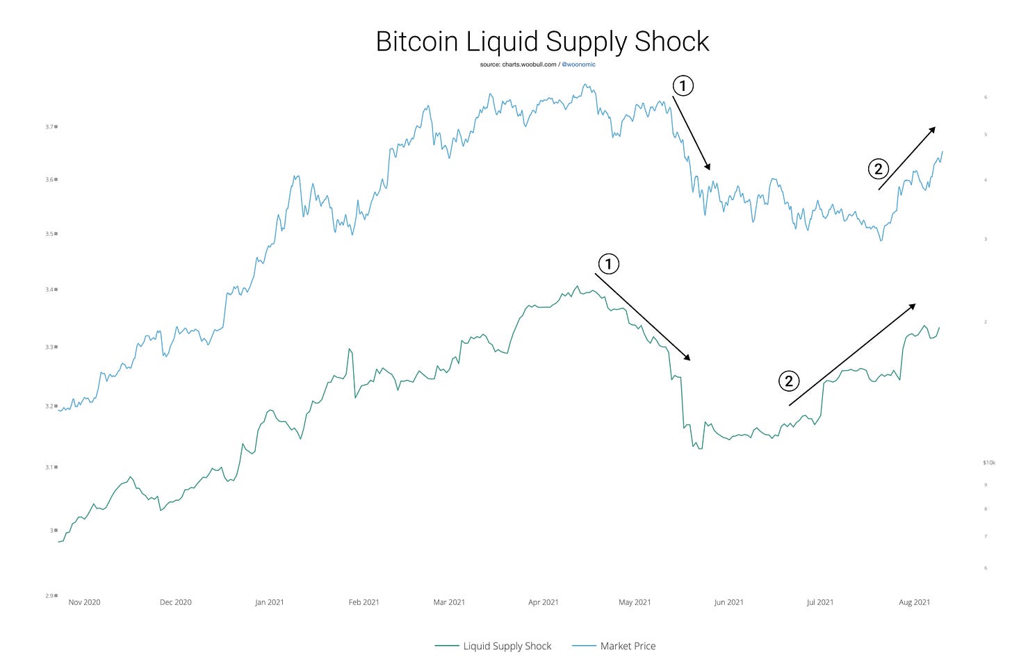
This makes sense as we are tracking the intent of investors BEFORE their action to buy or sell.
For example if a long term investor that historically accumulates moves enough coins to another entity (usually it’s to an exchange) all coins held by that investor become re-classified as liquid or highly liquid as the intent of the investor is now considered to have changed.
Here’s 3 different models of supply shock in the chart below with their equations.
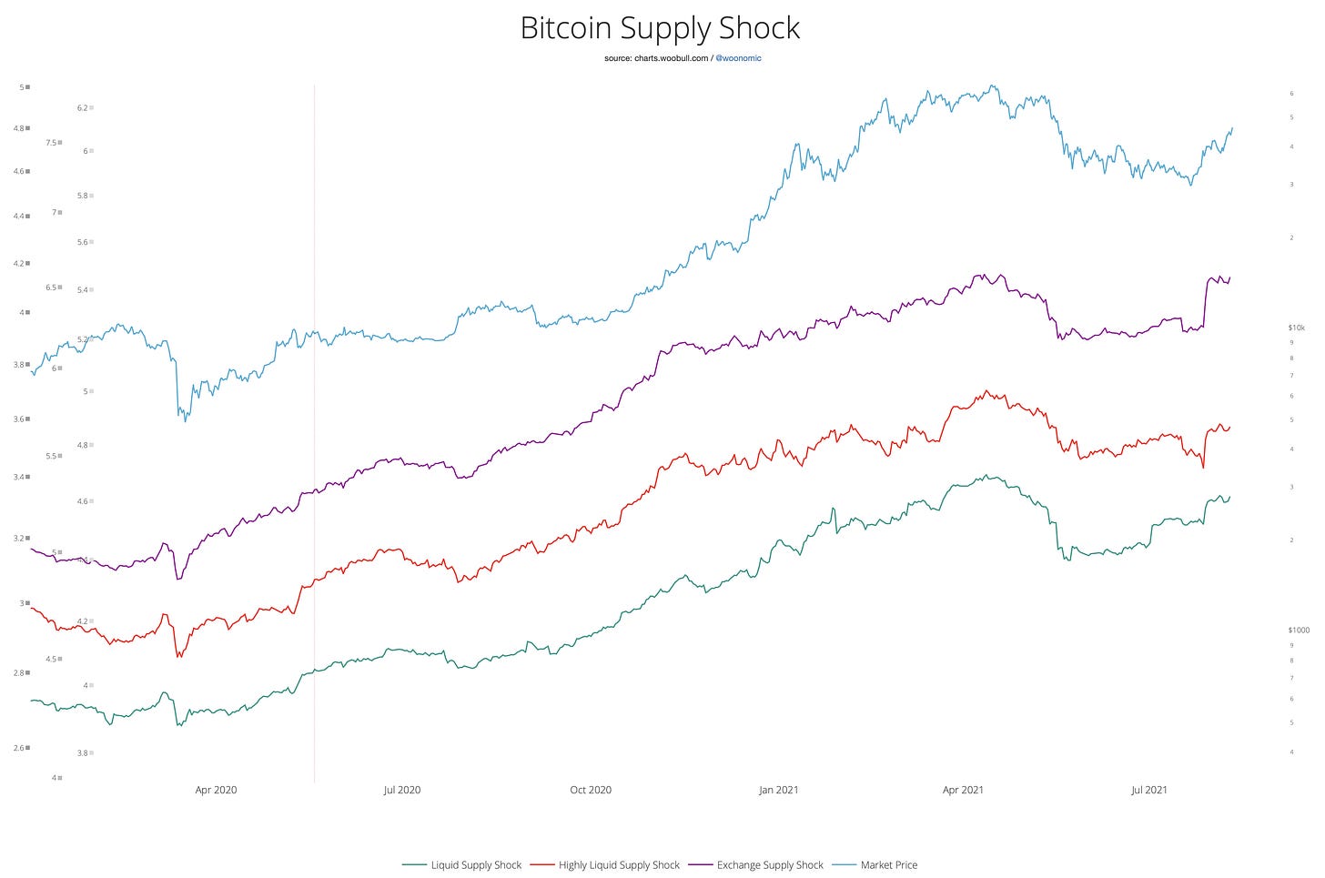
- Liquid Supply Shock (Green)
LSS = Illiquid Supply / (Liquid + Highly Liquid Supply)
Tracks coins held by long term investors vs coins held by speculators. - Highly Liquid Supply Shock (Red)
HLSS = (Illiquid + Liquid Supply) / Highly Liquid Supply
Similar to LSS but with emphasis on short term speculation activity. - Exchange Supply Shock (Purple)
ESS = Supply NOT on exchanges / Supply ON exchanges
Tracks coins in long term storage vs coins on exchanges that can immediately be sold.
Here’s another version of Supply Shock which looks quite different:
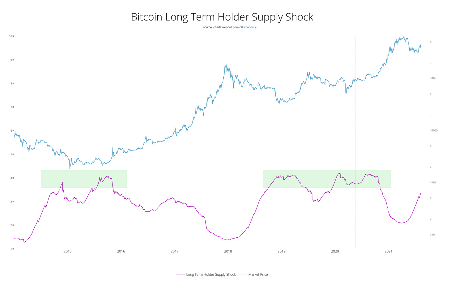
- Long Term Holder Supply Shock
LTHSS = Supply NOT moved in 155 days / Supply moved within 155 days
Since there’s a time window of 155 days delay before we get an indication of long term investment against short term speculation, this metric isn’t very responsive. Instead LTHSS provides a broader macro view of bull and bear phases of the market. LTHSS climbs higher in macro bottoms when sellers have been exhausted.
Note that 155 days (5 months) is a cut-off that Glassnode introduced to describe coins as part of the short term or long term supply.
Using Supply Shock in other asset markets
Obviously Supply Shock is not a property unique to Bitcoin. All asset markets will exhibit this property, however crypto-assets have the advantage of precise and real-time measurements.
Below is Ethereum’s Supply Shock.
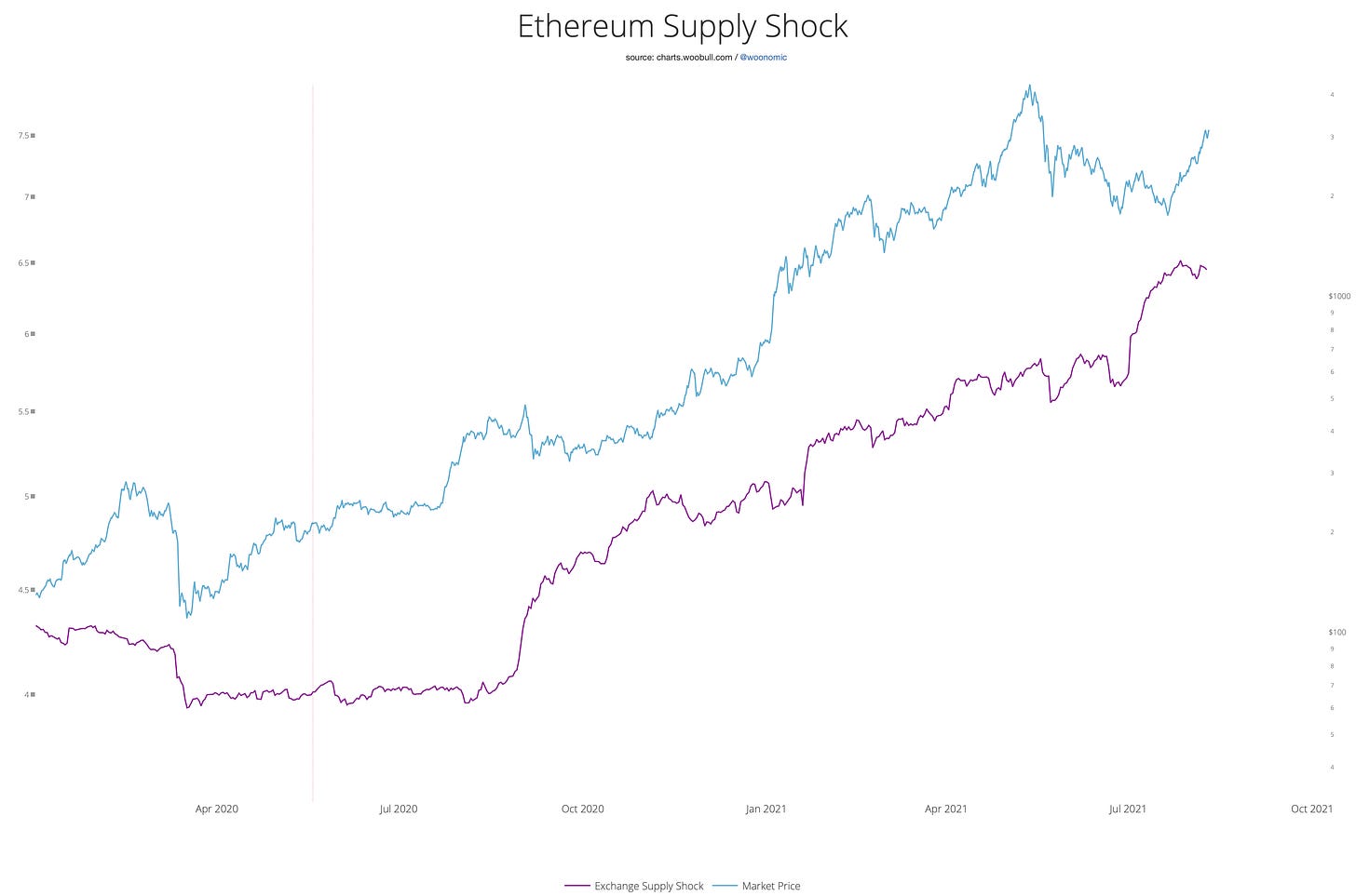
Modelling price using Supply Shock
In market conditions when the Supply Shock is within recent historical levels, it is possible to model a fundamental price.
We simply do a look-back on previous times the market had a similar Supply Shock and then find the array of prices the market recently assigned. I’ve done exactly this in the chart below using 3 methods of Supply Shock (LSS, HLSS and ESS).
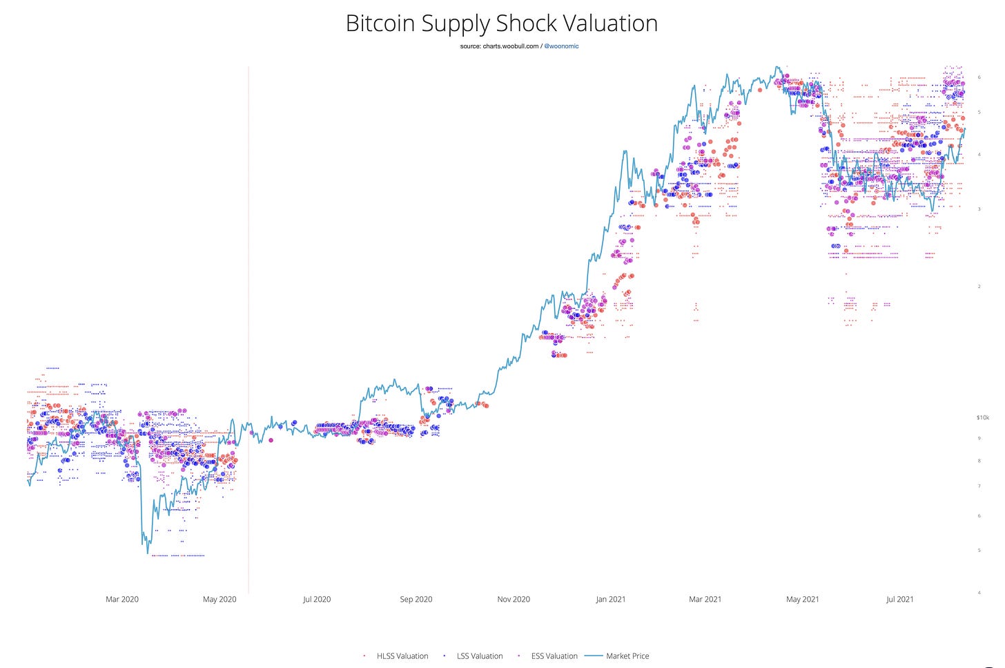
Small dots are prior valuations found, the larger dots are averages of those valuations. There are 3 colours representing each of the Supply Shock metrics respectively.
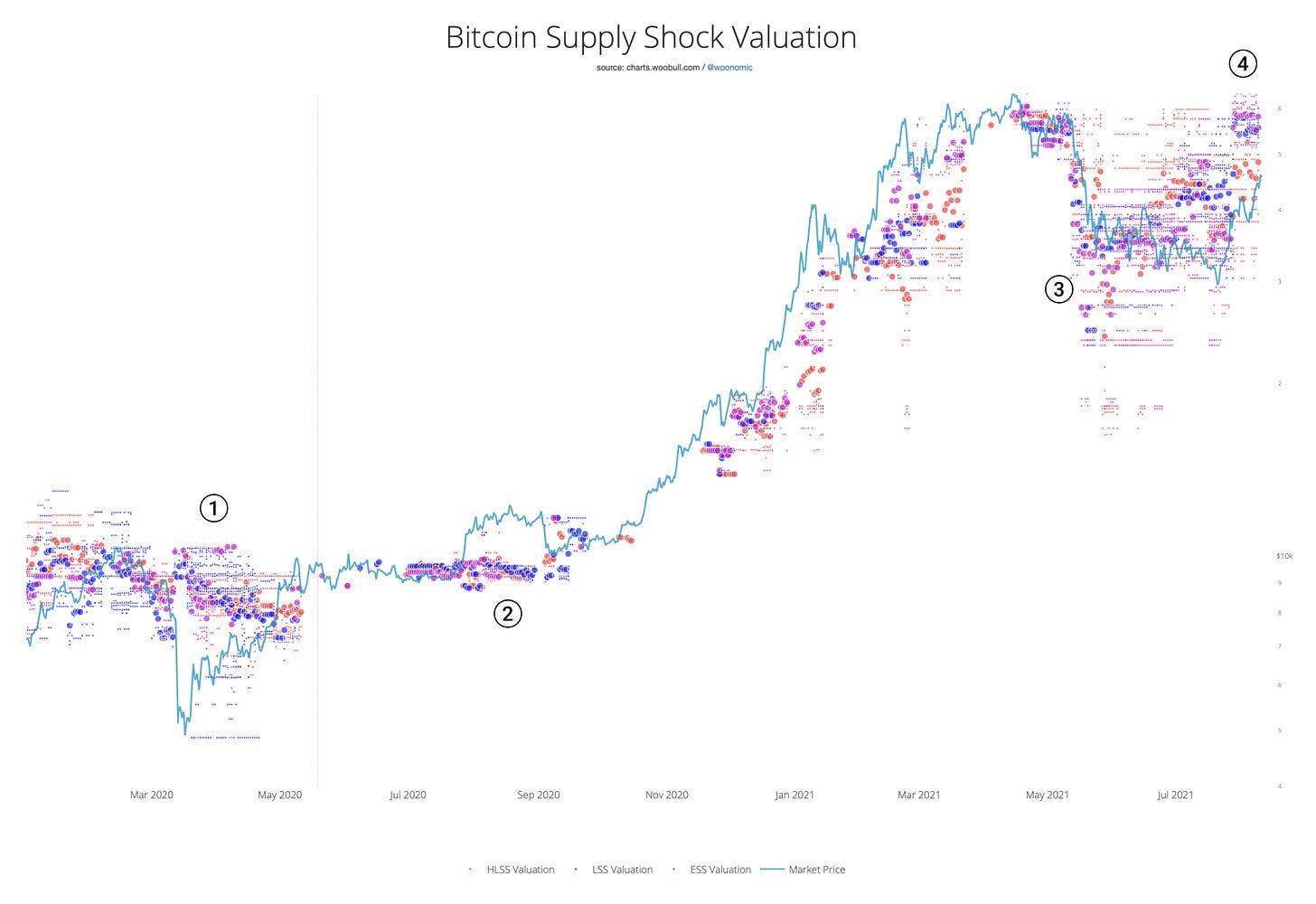
I’ve marked areas (1) and (2) where price (as determined by short term speculators) moved without any fundamental change in investor demand and supply. In these cases price reverted to the levels predicted by previous levels of supply shock.
In cases (3) and (4) the changes in investor demand and supply predicted and led price movements.
Conclusion
In this article I introduce the notion that intent to buy or sell can be quantified and used to predict a market’s future price movements. I present 4 methods to calculate this intent by estimating the supply that is not available against the supply that is available.
I demonstrate the resulting metric called Supply Shock can help predict price.
Furthermore using a look-back algorithm I show how under certain market conditions, where there is recent pricing data for a given supply shock value, a price target can be predicted.
Acknowledgements
Thanks to Will Clemente who was the first to suggest running a ratio between Glassnode’s Liquid Supply and Illiquid Supply. The results and subsequent investigations lead to this body of work.